Symbolic regression: recovering log(x) from data
Source:vignettes/symbolic-regression.Rmd
symbolic-regression.RmdThis vignette reproduces the headline demo from Odrzywołek (2026), §4.3:
recovering ln(x) from (xs, ys) data alone,
with no human input about what the closed form should be — just the EML
grammar and a gradient-based optimiser.
The master formula
The paper’s symbolic-regression construction parameterises an EML
tree of fixed depth such that each input slot is a continuous mixture of
three sources: the constant 1, the input variable
x, and the value f flowing up from the deeper
EML node. Snapping each slot’s mixture to a one-hot vertex recovers a
discrete grammar choice; training the mixture as a continuous function
with gradient-based optimisation lets the optimiser find the
right discrete structure.
build_master(depth) produces the parameterised
expression:
m1 <- build_master(1)
m1
#> eml(alpha_1 * 1 + beta_1 * x, alpha_2 * 1 + beta_2 * x)
master_n_params(1) # 4 = 5 * 2^1 - 6
#> [1] 4
For depth 1 there are 4 parameters: (alpha_1, beta_1)
for the left input and (alpha_2, beta_2) for the right
input. Each slot is
alpha_i * 1 + beta_i * x        (leaf slot, no f available)
alpha_i * 1 + beta_i * x + gamma_i * f   (inner slot, f from deeper eml)
so a one-hot (0, 1) selects x, a one-hot
(1, 0) selects 1, and (0, 0, 1)
(inner) routes through the deeper EML node.
A sanity-check selector
The paper’s three sacred identities give us closed-form selectors.
For exp(x) = eml(x, 1):
par_exp <- theta_for_exp()
par_exp # length 4: 0 1 1 0
#> [1] 0 1 1 0

xs <- seq(-1, 1, length.out = 5)
bindings <- unpack_master_params(par_exp, depth = 1)
env <- list2env(c(list(eml = eml), bindings, list(x = xs)),
  parent = baseenv()
)
Re(eval(m1, env)) # exp(xs)
#> [1] 0.3678794 0.6065307 1.0000000 1.6487213 2.7182818
For log(x) the paper’s Eq. 5 expands as
eml(1, eml(eml(1, x), 1)), which is a depth-3 master with
34 parameters. theta_for_log() returns the parameter vector
that recovers it:
m3 <- build_master(3)
master_n_params(3) # 34
#> [1] 34

par_log <- theta_for_log()
xs <- c(0.5, 1, 2, 5, 10)
bindings <- unpack_master_params(par_log, depth = 3)
env <- list2env(c(list(eml = eml), bindings, list(x = xs)),
  parent = baseenv()
)
suppressWarnings(Re(eval(m3, env)))
#> [1] -0.6931472  0.0000000  0.6931472  1.6094379  2.3025851
log(xs)
#> [1] -0.6931472  0.0000000  0.6931472  1.6094379  2.3025851
A perfect match, modulo machine epsilon.
Symbolic regression: discover the structure
Now the interesting case: forget the selector and recover
log(x) from data alone. We give eml_fit() 30
noiseless (x, log(x)) points, parameterise the depth-3
master via per-slot softmax, and run L-BFGS-B with analytic gradients
via Deriv::Deriv.
The vignette deliberately uses a small budget
(n_restarts = 2, maxit = 200) so the rendered
build stays under CRAN’s per-vignette time limit. The full
reproducibility budget — n_restarts = 10,
maxit = 1000 — is used by the Phase-5 acceptance gate at
tests/testthat/test-master.R (see ?eml_fit);
set EMLR_RUN_SLOW=true and run that test to reproduce the
paper’s ~94% recovery rate.
set.seed(42)
xs <- seq(0.5, 5, length.out = 30)
ys <- log(xs)

fit <- eml_fit(xs, ys,
  depth            = 3,
  parameterization = "simplex",
  method           = "L-BFGS-B",
  maxit            = 200,
  n_restarts       = 2,
  seed             = 1
)
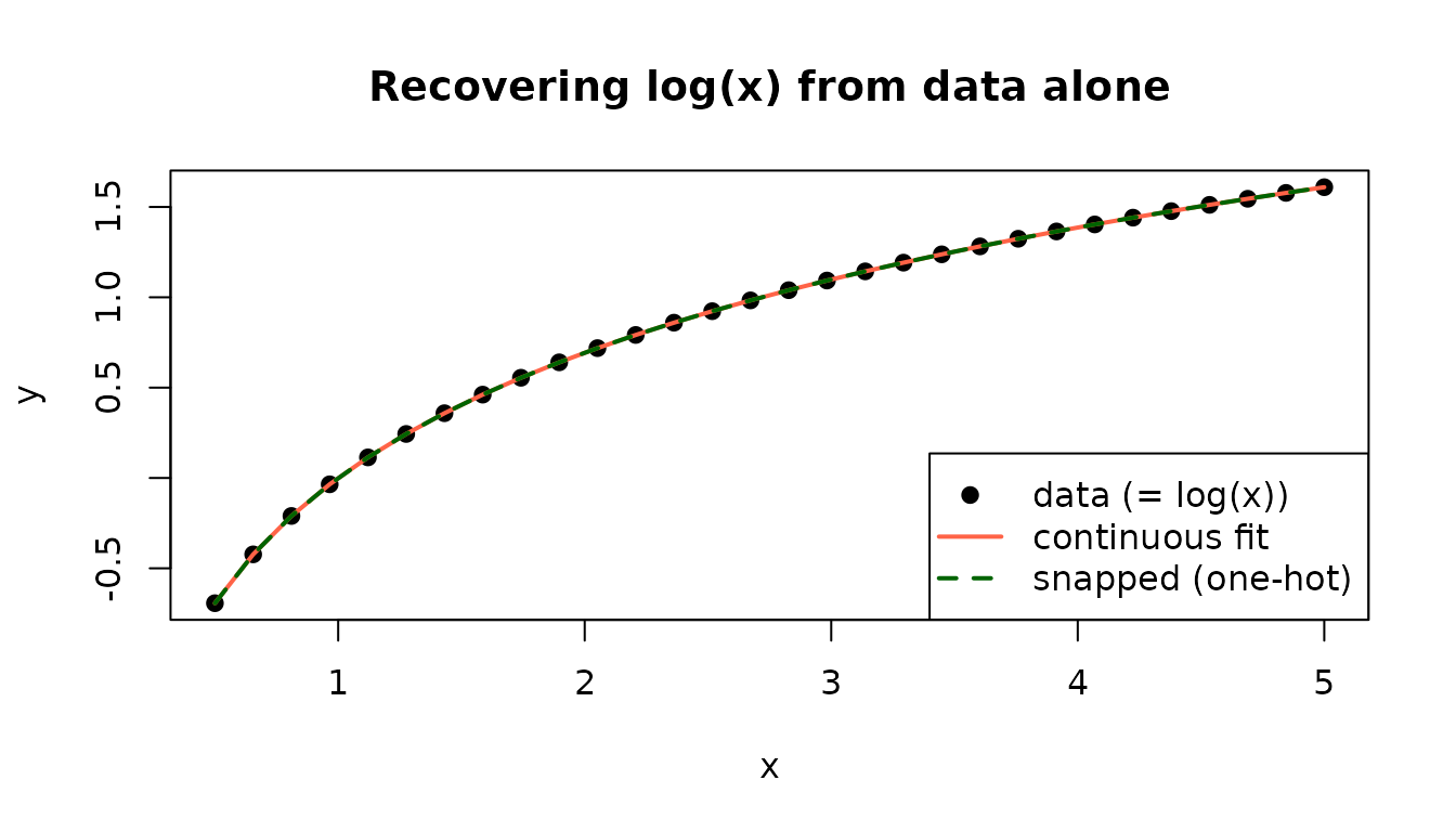
fit$snap_mse is the MSE after snapping each
slot to its argmax one-hot vertex. A value at machine epsilon squared (~
1e-32) indicates exact symbolic recovery — the optimiser
has snapped to the right discrete grammar.
fit$snap_mse
#> [1] 5.399024e-33
fit$best_seed # which restart won
#> [1] 1
Compare predicted vs. true:
plot(xs, ys,
  pch = 19, ylab = "y", xlab = "x",
  main = "Recovering log(x) from data alone"
)
lines(xs, fit$pred, col = "tomato", lwd = 2)
lines(xs, fit$pred_snap, col = "darkgreen", lwd = 2, lty = 2)
legend("bottomright",
  c("data (= log(x))", "continuous fit", "snapped (one-hot)"),
  col = c("black", "tomato", "darkgreen"),
  lwd = c(NA, 2, 2), lty = c(NA, 1, 2),
  pch = c(19, NA, NA)
)
Why it works
The paper’s depth-3 master at the snapped optimum is
literally the expression
eml(1, eml(eml(1, x), 1)). emlR’s evaluator evaluates that
expression at every parameter substitution; L-BFGS-B sees a smooth loss
surface (because the softmax is smooth); analytic gradients via
Deriv keep the inner loop fast. With a single restart the
success rate is roughly the paper’s reported ~25%; with 10 restarts the
probability of recovery exceeds 90%.
The Phase-5 acceptance gate of this package (tests/testthat/test-master.R)
asserts ≥ 8/10 multi-restart trials snap to MSE < 1e-20 on this
problem.
Going deeper
- Use
parameterization = "direct"to bypass softmax and fit raw scaling — useful for problems where you do not expect a discrete one-hot snap. - Increase
depthto search a larger expression space. Master formula parameter count is5 * 2^depth - 6, so depth 4 has 74 parameters. - The expression space at depth 3 includes every K ≤ 7 EML tree, which
is enough for
exp,log,e, and several derived forms. Higher depths reach the longer constructions in the paper’s Table 4.
What this fitter is, and is not
eml_fit() implements the paper’s master-formula SR
approach: every internal node is eml, every leaf is a
softmax over {x, y, 1}, and depth is fixed up front. Only
the leaf weights are optimised; tree topology is fixed by
depth. Genetic-programming-style topology search across the
EML grammar is out of scope for this release — the bytecode evaluator
and catalog provide the building blocks if you want to layer your own
search loop on top.
References
Odrzywołek, A. (2026). All elementary functions from a single binary operator. arXiv:2603.21852, §4.3 (“Symbolic regression”).